Recurrent Neural Network in Machine Learning

Recurrent Neural Network is a strong and durable sort of neural network, and is among the more intriguing methods still being used since they are the only ones that have internal memory.

Recurrent neural networks, like several other deep learning methods, are pretty recent. They were first developed in the 1980s, but we’ve only just realized their actual power. Growth in processing power, combined with the enormous quantities of information that we’ve had to deal with, as well as the advent of long short-term memory (LSTM) throughout the 1990s, has pushed RNNs to the forefront.

RNNs may recall critical details about the information they got due to their internal memory, allowing them to anticipate what will happen next with great accuracy. This is the reason they are the chosen method for time series, voice, textual, economic data, sound, film, meteorological, and many other types of sequential data. When opposed to other methods, recurrent neural networks can acquire a far richer knowledge of a series and its environment.

Why RNN:

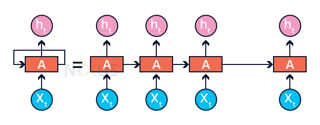
Conventional neural networks are unable to predict incoming input going by past ones. A typical neural network, for instance, cannot anticipate the next word in a series based on the preceding ones. A recurrent neural network (RNN) on the other hand, can. Recurrent neural networks, as their name implies, are recurrent neural networks. As a result, they run in loops, enabling the data to survive.

Types of recurrent neural network:

Recurrent Neural Networks are categorized as follows:

1. One to One RNN

This type of neural network is known as the Vanilla Neural Network. It’s used for general machine learning problems, which has a single input and a single output.

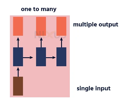
2. One to Many RNN

This type of neural network has a single input and multiple outputs. An example of this is the image caption.

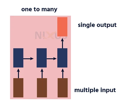
3. Many to One RNN

This RNN takes a sequence of inputs and generates a single output. Sentiment analysis is a good example of this kind of network where a given sentence can be classified as expressing positive or negative sentiments.

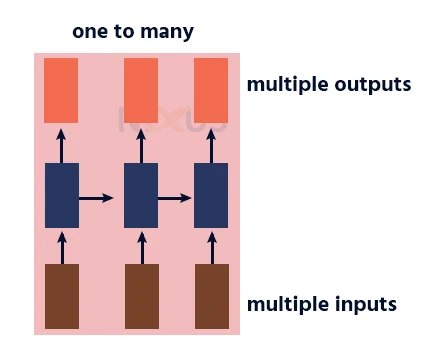
4. Many to Many RNN

This RNN takes a sequence of inputs and generates a sequence of outputs. Machine translation is one of the example.

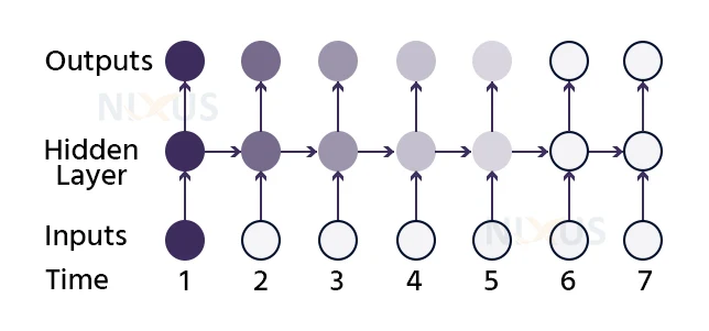
Recurrent Neural Network Architecture:

This is a more complex network with several hidden levels So, the input level gets the input, the first hidden state activations are performed, and these activations are then transferred to the next hidden units, and so on to form the result. Each hidden layer has its own set of values and biases.

Each layer behaves separately since it has its own values and activations. The goal is now to determine the link between consecutive entries. The weights and biases of these hidden layers differ in this case. As a result, all of these layers operates individually and it can be joined. To merge these hidden layers, we will use the same set of weights for these hidden units.

We may now merge these levels such that the values and biases of all hidden levels are one and the same. All of these hidden levels can be merged into a single recurrent layer.

As a result, it’s the same as providing input to the hidden layer. Because the recurrent neuron is now a solitary neuron, whose weight would have been the same at all time steps. As a result, a recurrent neuron remembers the state of a prior input and mixes it with the current, keeping some link between the current and past inputs.

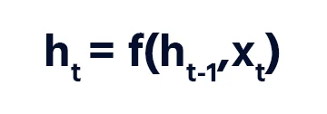
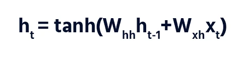
The formula for the current state can be written as:

And the activation formula can be given by:

Vanishing and Exploding Gradient Problem:

We use the chain formula above, but if one of the gradients approaches zero, the multiplier causes all of the gradients to race to zero exponentially rapidly. Such conditions will no longer aid the network’s learning. This is referred to as the vanishing gradient problem.

The vanishing gradient dilemma is significantly more dangerous than the bursting gradient problem, in which gradients grow extremely huge because of such an instance or numerous gradient values getting incredibly high.

The solution to the gradient problem is agreed to be long term short memory networks. They help solve issues that arise from there being a gap between relevant information and application of the same.

What is LSTM?

Long short-term memory networks (LSTMs) are a type of recurrent neural network extension that essentially increases memory. As a result, it is highly adapted to learning from significant events that have very lengthy period delays between them. The components of an LSTM are utilized to construct the layers of an RNN, which is also known as an LSTM system.

RNNs can recall inputs for a lengthy distance because of LSTMs. This is due to the fact that LSTMs store data in a memory, similar to a computer ‘s memory. The LSTM has the ability to receive, update, and erase data from its cache. This memory may be thought of as a normal cell, where the unit selects either or how to retain or erase data (i.e., whether or not to open the gates) based on the value it attributes to the data. Weight values are used to indicate significance, which are also learnt by the method. Knowledge is valuable and the machines gain it over time.

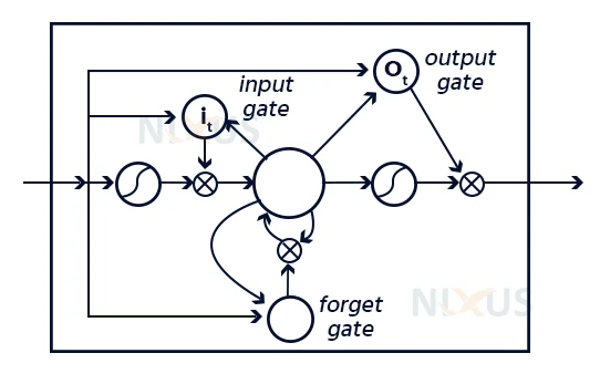
Working of LSTM:

LSTMs work in three stages with clearly defined formulae for each stage

The initial stage in the LSTM is to select whether data from the unit must be excluded in that time step. This is determined by the sigmoid function. It calculates using the prior state (ht-1) and the input data xt.

There really are two elements to the second level. The sigmoid function determines which variables are allowed to pass (0 or 1). The tanh function assigns value to the items supplied, determining their relative significance (-1 to 1).

The third stage is to determine what will be the result. We start with a sigmoid layer, which determines whether aspects of the cell state make the final stage.

What is GRU?:

The Gated Recurrent Units, or GRUs, are also one effective RNN design. Those are similar to LSTMs but have fewer components and are better to handle. Their effectiveness is largely due to the gating network signals, which govern how the existing input and past memory are used to change the existing activation and generate the current scenario. During the training phase, these gates have their own sets of weights that are adaptively changed. There are just two gates here: the reset and the update gates.

Working of Recurrent Neural Network

A hidden layer that has its own collection of weights exists in classic neural nets. Let’s call this value and bias w1 and b1, respectively. We’ll have w2,b2 and w3,b3 for the third step, too. These layers are likewise self-contained, which means they don’t remember the preceding result.

Consider a more complex network with one input layer, three hidden levels, and one output layer. The recurrent network converts independent activations into dependent activations first. It also gives all the layers the same weight and bias, simplifying RNN variables and providing a consistent foundation for remembering past outputs. The 3 component layers aggregate into one recurrent unit with the very same weights and bias.

Training through RNN:

• The system only accepts one time step of the inputs.
• The present state may be calculated using the input signal and the prior condition.
• Now, for the next state,the present state through ht-1.
• There are n steps, and at conclusion, all of the data may be connected.
• The last phase is to calculate the result once all of the processes have been completed.
• Finally, we calculate the deviation by subtracting the correct performance from the expected value.
• The mistake is back propagated to the network, where it is used to change the weights and provide a bigger return.

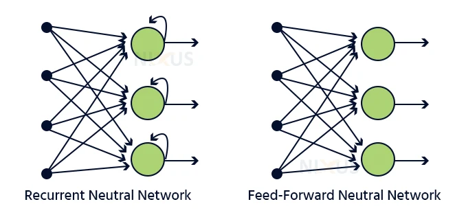
Feed-forward vs RNN:

The data in a feed-forward neural network only goes in one path: from the inner to the outer layer, via the hidden layers. The data travels in a straight line through the network, never touching a component again.

Feed-forward neural networks really had no recollection of the input and are lousy at guessing what will happen next. A feed-forward network has no concept of time order since it only analyses the present input. It simply cannot recall anything from the past other than its own instruction.

The data in an RNN cycles via a loop. When it reaches a judgment, it takes into account the current input as well as what it has learnt from prior inputs.

RNN issues:

1. Exploding gradients:

Exploding gradients occur when the algorithms gives the weights an absurdly high priority for no apparent reason. However, truncating or suppressing the gradients is a simple solution to this issue.

2. Vanishing gradients:

Because when coefficients of a gradient are too tiny, the algorithm ceases training or requires far too much time to learn. This was a huge issue that was far more difficult to overcome than the exploding gradients. Thankfully, Sepp Hochreiter and Juergen Schmidhuber’s LSTM idea addressed the problem.

Backpropagation:

Whenever you implement a Backpropagation method to a Recurrent Neural Network with time series data as its feed, we call it backpropagation over time.

A single input is sent into the system at once in a conventional RNN, and a single output is generated. Backpropagation uses both the previous and present inputs as input. This is referred to as a time – step, and one timestep will comprise of multiple time series data points in the RNN at the same moment.

Applications of Recurrent Neural Network

Picture labeling, text categorization, machine translation, and sentiment classification all make extensive use of RNN. For instance, a film review can help you comprehend how the viewer felt after viewing the film. When the film studio does not have enough time to evaluate, aggregate, categorize, and analyze the evaluations, automating this operation comes in handy. The machine can perform the task with more precision.

1. Speech recognition:

Conventional language processing techniques based on Hidden Markov Models have been supplanted by Recurrent Neural Networks. Such Recurrent Neural Networks, in conjunction with LSTMs, are more suited for identifying speeches and translating them into writing without losing meaning.

2. Sentiment analysis:

We employ emotion research to determine if a statement is positive, negative, or indifferent. As a result, RNNs are best at handling input consecutively in order to discover sentence emotions.

3. Image tagging:

RNNs, in combination with convolutional neural networks, can identify pictures and generate labels to describe them. An image of a fox leaping more than a wall, for instance, is best conveyed using RNNs.

Benefits of RNN

• An RNN retains each piece of information it encounters over duration. This is only effective in time series forecasting due to the sheer ability to recall past inputs. This is referred to as Long Short Term Memory.
• To obtain a greater pixel neighborhood, recurrent neural networks are combined with convolutional layers.

Limitations of RNN

• Issues with gradients disappearing and exploding.
• It is quite tough to program an RNN.
• When utilizing tanh or relu as an activation function, it could perhaps parse very short sequences.

Conclusion

In this article, we have explained to you what an RNN is, how it works, its types and how it is different from other models. We have also laid out the advantages and disadvantages of the same. Hope this will help you to get a basic theoretical understanding and to see if RNN is the right fit for your project.