Types of Learning Rules in ANN
The functioning of the human brain serves as the inspiration for artificial neural networks (ANN). Consider the mammalian central nervous system. The capacity to adjust is indeed the biological body’s greatest skill, and ANN develops comparable traits. You ought to comprehend how precisely our brain works. Even if we possess a basic grasp of the process, it is still relatively crude. Studies claim that the architecture of the human brain changes in the process of learning. These changes occur in connections between neurons, where the strength of the connection changes depending on how active they are.
Artificial neural networks: similarity to the human body
By altering the valued linkages existing among nodes in the network, ANN may simulate human cognitive development. It successfully reflects the enlarging and contracting of the connections between neurons in our brain. The development and disintegration of the connections enable the system to adjust. Recognition software is an example of a situation that would be very challenging for a person to translate accurately into a script.
A bank or financial organisation using past credit ratings to categorise potential lending possibilities is a problem that a machine learning model can address effectively. Training an ANN is the process of teaching a processing element to alter its behaviour in reaction to any change in its surroundings. When a specific system is built, the fixed activation function and input/output vector improve the significance of training in ANN. We must now modify the weighting to alter the input and output behaviour.
What are ANN Learning Rules?
A method or mathematical problem known as the learning rule promotes a neural network to benefit from its current situation and improve efficiency. Moreover, it is a repetitive process. We will discuss the learning rules in neural networks in this lesson. The mathematical formulae for all of these rules are given here.
A strategy or logic is referred to as a learning rule. It applies this rule throughout the network and enhances the efficiency of the artificial neural network. Thus, when networks replicate in a new environment, learning rules update the weights and bias values of the network.
Types of ANN Learning Rules
We know that changing the parameters during ANN training will modify the input/output behaviour. Therefore, we need a system that allows us to modify the weights or values in each learning process step. Such techniques, which are merely procedures or formulae, are known as learning rules. The neural network’s training guidelines are listed below.
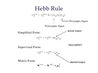
1. Hebbian learning rule
The fundamental guideline for knowledge is the Hebbian principle. Donald Hebb developed this unsupervised neural network-based approach in 1949. We can use this formula to increase a network’s node weight.
According to the Hebb learning rule, the weight attached to the nearby neurons will rise if they are both engaged and deactivated simultaneously. Conversely, the weight of neurons operating at opposing stages should decrease. The weight should not vary when there is no link between the input signal. The mathematical formula for Hebb’s learning rule is given below:
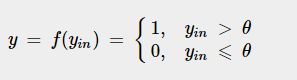
2. Perceptron Learning Rule:
A neural network’s connections all have a value that varies as the network learns. It claims that as an illustration of supervised learning, the network begins its learning process by giving each value a random number.
Determine the output value based on a collection of records for which we know the anticipated output value. The learning example that gives the full definition is this. It is referred to as a learning example as a consequence.
The system then matches the estimated output value to the anticipated value. Finally, the sum of the squares of the mistakes that occurred for each person in the learning sample may be used to build an error function, which is the next step.
This is an instance of supervised methods since the weight of the vertices is assigned as per consumers.
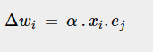
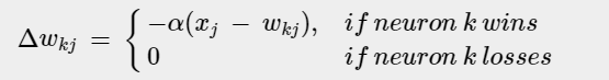
3. Delta Learning Rule:
The Delta rule is a popular learning principle that Widrow and Hoff created. It depends on supervised methods. According to this rule, the combination of the errors and the inputs alters a network node’s weight.
The delta rule is expressed mathematically as follows:
We compare the output to the input to determine the proper response. If the gap is zero, no knowledge is acquired; if the gap is greater than zero, we need to adjust the values to get a zero gap. Use the delta rule to form random connections if the collection of input patterns forms an isolated set.
For systems with linear activation factors and no hidden units, the delta learning rule may be used for both solitary and the presence of multiple units.
Assuming that the mistake can be accurately quantified when using the delta rule.
The delta rule seeks to minimise inaccuracy, which we can define as the difference between the output that was produced and what was anticipated.
4. Correlation Learning Rule
The Hebbian learning rule and the correlation learning rule both operate on the same fundamental ideas. It assumes that values should vary in relation to cell response. That is, values between responsive cells need to be more positive. The inverse is also true where values between cells that react opposingly are more negative.
The correlation rule is indeed the supervised machine learning algorithm, which is the opposite of the Hebbian rule.
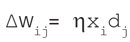
5. Out Star Learning Rule
If the nodes or neurons in a system are organised in a layer, you apply the OutStar Learning Rule. In this case, the values attached to a particular node are identical to the expected outputs for the cells linked via those weights. This rule generates the required output for the layer of n nodes in the network, t.
Use this kind of training for each node in the level in question. The node values have been updated to match those in Kohonen neural nets. Write the out star learning in quantitative form like:
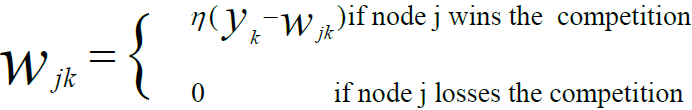
6. Competitive Learning Rule
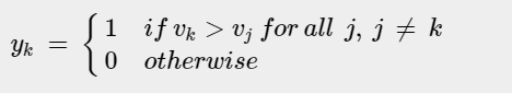
A competitive learning rule has a group of identical neurons except for a few synaptic weights distributed unequally. So they respond differently to a specific set of inputs. A restriction is placed on each neuron’s “strength.” It is associated with unsupervised learning, where the output nodes battle to match the input sequence. The output unit with the greatest activation value to an input data sequence will be considered the winner throughout training.
This rule is also known as the winner-takes-all rule since only the winner neuron is modified while the remaining neurons remain untouched.
This rule has three conditions (or rules) that are represented by mathematical formulae:
Condition under which winner is selected:
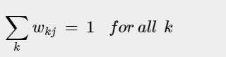
The Condition for the total sum of weights:
Condition for the change in weight of the winning neuron
Conclusion
The capacity of the Artificial Neural Network to learn is one of the most intriguing aspects of the system. The brain’s neuronal architecture changes as a result of learning. Their neural interconnections might get stronger or weaker depending on how busy they are. Stronger synaptic connections are made by more pertinent knowledge.
As a result, there exist several strategies for developing artificial neural networks. Each one has advantages and disadvantages. In addition to these learning guidelines, machine learning algorithms can also learn through supervised, unsupervised, and reinforcement learning. Back Propagation, ART, and Kohonen Self Organizing Maps are some popular ML techniques.