Consumer Credit Risk Prediction Machine Learning Project
With this Machine Learning Project, we develop a consumer credit risk prediction system. For this project, we use Random Forest Classifier, easy ensemble classifier model.
So, let’s build this system.
Consumer Credit Risk
Banks incur significant losses due to their clients’ defaulting on their loans, but ultimately it is ordinary people who suffer the most due to this error. The banks utilize credit risk analysis to ensure that the credit is given to a trustworthy customer.
Credit risk is the possibility of defaulting on a loan due to the borrower’s failure to make the necessary debt payments on schedule. The lender assumes this risk because failure to do so could result in both principal and interest losses.
The onerous human task of examining different criteria and requirements on which credit can be granted is eliminated by credit risk analysis utilizing machine learning. Additionally, it eliminates human corruption and mathematical inaccuracy from the process. In this instance, we are dealing with a bank that serves as the financial institution disbursing loans to clients who request them.
Customers who might miss a loan payment are therefore credit risks for the bank. The bank will be able to detect in advance whether customers might be potential credit risks by evaluating customer data and using machine learning algorithms on it. Preventing loans from being extended to clients who might pose credit issues to the bank, will aid in risk mitigation and loss minimization.
In this study, we suggest a cardinal measure of consumer credit risk that combines classic credit variables, including debt-to-income ratios, with consumer banking activities which significantly increases the prediction power of our model.
We demonstrate that conditioning on specific changes in a consumer’s bank-account activity can result in significantly more accurate forecasts of credit-card delinquencies in the future using a proprietary dataset from a major commercial bank, which we shall refer to as the “Bank” throughout this project, to preserve confidentiality. For instance, in our sample, the unconditional probability of customers becoming 90 days or more past due is 5.3%, but customers who have recently experienced a decline in income—as indicated by sharp drops in direct deposits—have a 10.8% probability of becoming 90 days or more past due over the ensuing six months.
Our method can produce a variety of these transaction-based predictors and combine them nonlinearly with credit bureau data to provide even more potent forecasts. These conditioning variables are statistically reliable over the whole sample period. We are able to spot small nonlinear associations that are challenging to spot in these enormous datasets when using conventional consumer credit-default models like logit, discriminant analysis, or credit scores by examining patterns in consumer spending, savings, and debt payments.
We employ a strategy known as “machine learning” in the literature on computer science, which describes a collection of algorithms created especially to address computationally demanding pattern recognition issues in very sizable datasets.
Due to the large sample sizes and the complexity of the potential relationships between consumer transactions and characteristics, these techniques—which include radial basis functions, tree-based classifiers, and support-vector machines—are particularly well suited for consumer credit risk analytics. Our consumer credit-risk model is only one recent example of the renaissance in computer modeling brought about by the remarkable speedup in computing in recent years along with major theoretical developments in machine learning methods.
Random Forest Classifier
The family of ensemble learning algorithms includes random forests, commonly referred to as random decision forests, which are machine learning algorithms. It is utilized for both classification and regression problems. The name “random forests” refers to nothing more than a grouping or ensemble of decision trees. It employs numerous decision trees, each of which is dependent on a specific dataset with a consistent distribution throughout the tree. In a class population of unbalanced data sets, this model effectively balances errors. It can be applied to resolve classification and regression issues.
For classification, regression, and other problems, the random forest or random decision forest, uses several decision trees during the training phase. For categorization issues, the majority of trees opt for the random forest’s output. For regression tasks, the mean or average forecast of each individual tree is returned. Random choice forests correct the tendency of decision trees to overfit their training set. Random forests are less precise than gradient-boosted trees despite frequently outperforming them. However, data anomalies may reduce their usefulness.
Using the OOB data, random forests also construct a distinct variable important measure, to evaluate the predictive potential of each variable. As the bth tree develops, the OOB samples are sent down it, and the prediction precision is recorded. After the t values for the jth variable have been randomly permuted in the OOB samples, the accuracy is once more determined. The relevance of variable j in the random forest is assessed by applying the average accuracy loss caused by this permuting to all trees. Despite the similarities in ranks between the two methods, the importance is more evenly spread across the variables in the right plot. Randomization essentially nullifies the impact of a variable, similar to setting a coefficient in a linear model to zero. This does not measure the influence on prediction where it is unavailable because other variables might be used as holds if the model were updated without the variable.
Project Prerequisites
The requirement for this project is Python 3.6 installed on your computer. I have used a Jupyter notebook for this project. You can use whatever you want.
The required modules for this project are –
- Numpy(1.22.4) – pip install numpy
- Tensorflow(2.9.0) – pip install TensorFlow
- OpenCV(4.6.0) – pip install cv2
That’s all we need for our project.
Consumer Credit Risk Prediction
We provide the dataset and source code for this consumer credit risk prediction project that we require later in this project. Please download the dataset and code from the following link: Consumer Credit Risk Prediction Project
Steps to Implement
1. Import the modules and the libraries. For this project, we are importing the libraries numpy, pandas, and sklearn.
import numpy as np #importing the numpy library
import pandas as pd#importing the pandas library
import matplotlib.pyplot as plt#importing the matplotliblibrary
import seaborn as sns#importing the seaborn library
from pathlib import Path#importing the pathlib library
from collections import Counter#importing the collections library

from sklearn.metrics import balanced_accuracy_score#importing the sklearnlibrary
from sklearn.metrics import confusion_matrix#importing the confusion matrix
from imblearn.metrics import classification_report_imbalanced#importing the classification report library
2. Here we are importing the important columns of our dataset.
target = ["loan_status"] #creating the target variable as loan status
3. Here we are loading our dataset and we are dropping some unnecessary components from the dataset.
file_path = Path('dataset.csv')#loading the dataset
df = pd.read_csv(file_path, skiprows=1)[:-2]#reading the dataset using pandas

df = df.dropna(axis='columns', how='all') #dropping all the columns where there is any null value

df = df.dropna() #dropping all the null rows

issued_mask = df['loan_status'] != 'Issued' #here we are removing the issued load status columns

df['int_rate'] = df['int_rate'].str.replace('%', '')#here we are removing the percentage sign
df['int_rate'] = df['int_rate'].astype('float') / 100#here we are converting it to float value


x = {'Current': 'low_risk'} #here we are converting the current to low risk
df = df.replace(x) #here we are making changes in our dataset

x = dict.fromkeys(['Late (31-120 days)', 'Late (16-30 days)', 'Default', 'In Grace Period'], 'high_risk')#here we are converting the current to low risk
df = df.replace(x)#here we are replacing in the dataset

df.reset_index(inplace=True, drop=True)#here we are resetting the index values

df.head()#here we are printing our dataset
4. Here we are creating our features from the dataset.
X_df = df.drop(columns=['loan_status'])#here we are dropping the column loan status
X = pd.get_dummies(X_df,)

y = df['loan_status'].to_frame()#here we are creating our target dataset.
5. Here we are splitting the dataset into testing and training dataset.
from sklearn.model_selection import train_test_split#importing the train test split

X_train, X_test, y_train, y_test = train_test_split(X, y, random_state=1, stratify=y)#dividing the dataset into training, testing
6. Here we are defining our Random Forest Classifier model and we are scaling the data. After this, we are training the dataset and we are fitting our training dataset.
from sklearn.preprocessing import StandardScaler

scaler = StandardScaler() #creating an instance of standard scalar
X_scaler = scaler.fit(X_train)#here we are fitting our x dataset
X_train_scaled = X_scaler.transform(X_train)#here we are transforming the dataset
X_test_scaled = X_scaler.transform(X_test)#here we are transforming the dataset

from imblearn.ensemble import BalancedRandomForestClassifier#improting the balanced Random Forest Classifier

brfc = BalancedRandomForestClassifier(n_estimators =1000, random_state=1)#creating an instance of balanced forest classifier
model = brfc.fit(X_train_scaled, y_train)#fitting the model with the dataset
7. Here we are calculating the balanced accuracy score.
predictions = model.predict(X_test_scaled) #here we are passing the dataset and we are predicting the model
accuracy_score(y_test, predictions)#calculating the accuracy score

confusion_matrix(y_test, predictions) printing the confusion matrix
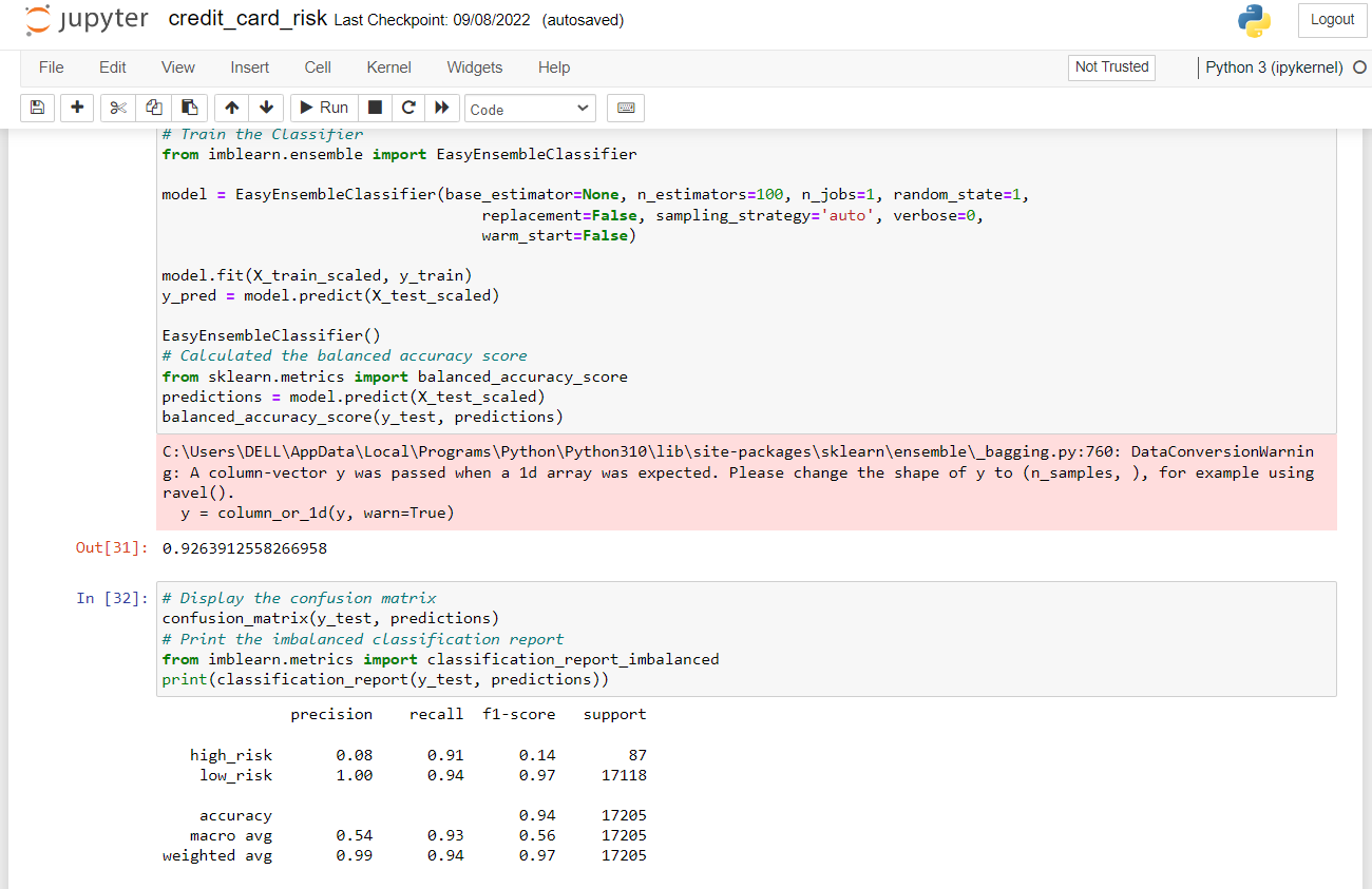
8. Here we are creating the easy ensemble classifier and then we are calculating the balanced accuracy score.
from imblearn.ensemble import EasyEnsembleClassifier

model = EasyEnsembleClassifier(base_estimator=None, n_estimators=100, n_jobs=1,)#here we are creating an instance of easy ensemble classifier

model.fit(X_train_scaled, y_train) #here we are fitting our moel with the dataset

predictions = model.predict(X_test_scaled)#predicting the value of the testing dataset
balanced_accuracy_score(y_test, predictions)#calculating the balanced accuracy score

confusion_matrix(y_test, predictions)#printing the confusion matrix
Consumer Credit Risk Prediction Output
Summary
We built a credit risk prediction system machine learning project. We have used Random Forest Classifier and an easy ensemble classifier model for this project. We hope you have learned something new from this project.