Gaussian Mixture Model
In this article, we will learn about Gaussian Mixture Model in machine learning. Let’s start!!
Introduction to Gaussian Mixture Model
Machine learning (ML) is the analysis of computer systems that can understand and develop on their own with expertise and input. In ML, sometimes we have problems that require us to divide a dataset into a number of groups or clusters. This is clustering. Clustering has a variety of approaches, including:
- K Means Clustering
- Hierarchical Clustering
- Distributive clustering
The chance of an item getting used in a distribution diminishes as the range among it and the main dispersion of points grows in distribution-based clustering.
The Gaussian distribution method is used to solve issues like these. The Gaussian model operates like this: there will be a specific amount of distributors. From the interior to outside, these distributors are concentric circles with diminishing color.
Because we now have larger distributors, the middle section tends to be dense, and it begins to diminish as we get outside. As a result, even if distributors contain the very same amount of points, their density may vary according to distributor length. For this form of grouping, overfitting can be a concern.
Gaussian Distribution model
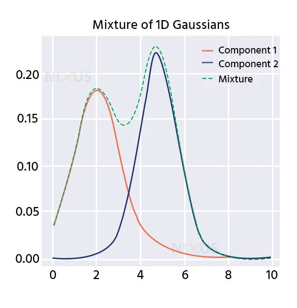
To simulate real-life datasets with bias in mean and variance values we use Gaussian Distribution (Univariate or Multivariate). The datasets are symmetrically distributed around the mean value, giving the curve shape of a bell. As a result, it is reasonable and straightforward to infer that the clusters are from various Gaussian Distributions. Or, to put it another way, the data is being modeled as a blend of many such distributions. This is the central concept.
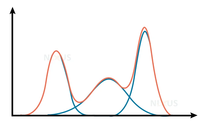
A few of these Gaussian distributions are shown below:
Choice of initialization:
To produce the starting centers for the model parameters, you may use one of four initialization approaches (along with entering user-defined starting means):
k-means (default)
It uses the classic k-means clustering technique. When contrasted to alternative initialization approaches, this can be relatively costly.
k-means++
This employs the k-means++ initialization approach for clustering. This will select the first center from the data randomly. Following centers will be picked using a weighted distribution of the data, with locations farther distant from previous centers being preferred. The usual initialization for k-means is k-means++, which is faster than executing a complete k-means but nevertheless takes a long time for big data sets with different parts.
random from data
As starting centers, this will select random sets of data from the supplied data. This technique of initialization is relatively quick, but it might generate non-convergent outcomes if the selected spots are too near together.
random
The centers are selected as a slight deviation from the data’s average. This strategy is straightforward, but it may cause the algorithm to take more time to converge. We can prevent overfitting as far as we don’t specify any strict point criterion.
The expectation-maximization model is frequently combined with the Gaussian mixture technique. It’s vital to recall that we can’t utilize this strategy for density-based clustering since the ranges wouldn’t fit well.
Expectation-Maximization approach:
The statistical approach Expectation-Maximization (EM) can identify the best hyperparameters. When there are discrepancies in the data, or when the data is partial, we usually employ EM.
Latent factors are variables that are absent from a dataset. When dealing with any unsupervised learning issue, we take the number of clusters to be uncertain. Owing to incomplete data, determining the correct model parameters is challenging. Consider the above: if you know which object belonged to which cluster, determining the mean vector and covariance matrix would be simple.
Difference between GMM and K-Means:
| Gaussian Mixture Model | K-Means |
| More versatile but also more complicated to train | Cannot serve too many purposes but is simple enough to train |
| High running time requirement | Faster to train and requires low running time |
| Makes assumption that each data point originates from a combination of Gaussian distribution | Makes no assumptions.Simply partitions data into clusters |
| Takes variance into account | Does not tackle variance at all. |
| More effective as they can handle missing values | Cannot handle missing data so resources will be need to clean or augment data |
| Shape of the clusters is flexible and can be changed | Limited to spherical clusters |
| More accurate for small datasets and clusters that aren’t distinct | More accurate when dataset is large with distinct clusters |
Key steps:
1. Covariance matrix:
We create a covariance matrix to numerically represent the relation between two Gaussians. The closest two Gaussians in terms of likeness have the closest their means and vice versa. The matrix can be diagonal or symmetric also
2. Clusters:
We decide the number of clusters by the number of Gaussians.
3. Hyperparameters:
We choose the hyperparameters that specify how to use GMMs to best segregate data.
Scenarios where Gaussian Mixture Model is useful
Whenever information is captured by a combination of Gaussian distributions, whenever there is ambiguity about the right number of clusters, and when said clusters have varied forms, Gaussian mixture models can be utilized. The adoption of a Gaussian mixture model can assist increase the accuracy of findings in each of these scenarios.
Some other scenario is when a collection has several groups that are difficult to categorise as pertaining to either one, making it very difficult for machine learning techniques like the K-means clustering algorithm to segregate the data. In this scenario, GMMs may be employed since they determine the optimum Gaussian mixture models for each cluster and offer a probability for each group, which is useful for naming clusters.
Gaussian mixture models may be used to produce synthetic data points that are comparable to the actual data, as well as data augmentation.
Applications of GMM
1. Medicine:
Finding patterns in medical datasets: GMMs may be used to categorize photos based on their content or to detect particular patterns in medical datasets. They may be used to detect illness, detect groups of people with common complaints, and perhaps even make predictions.
2. Natural phenomena:
GMM can be applied to represent natural processes in which noise is observed to match Gaussian distributions. This bayesian modeling paradigm is based on the idea that there is an underneath spectrum of unseen objects or qualities, each of which is linked to observational data performed at equidistant places throughout numerous test sessions.
3. Consumer behavioral analysis:
GMMs may be used in advertising to undertake user behavior analysis and generate forecasts based on previous data regarding possible potential transactions.
4. Stock price prediction:
Stock price prediction is yet additional use of Gaussian mixture models, which may be utilized to a stock’s price time – series data in economics. GMMs may be employed to identify changepoints in time series analysis and aid in the discovery of stock price pivotal moments or other market moves that would normally be impossible to notice owing to instability and chaos.
5. Study of gene sequences:
Gaussian mixture models may be used to analyze genetic data. GMMs may be used to find genes that are differently regulated across two circumstances and determine which proteins may relate to a certain phenotypic or disease condition.
6. Audiovisuals:
GMMs have lately been shown to extract the features from audio data for use in speech recognition systems. They are also significant in tracking multiple objects, where the amount of components in the mixture and values of their means anticipate where an object will be located in every frame in a video. The EM method keeps updating the element average as the frames keep changing, allowing us to track objects.
Advantages of Gaussian Mixture Model
1. Automatic selection:
When the weights are minimal and we have a large number of components, the Variational Bayesian mixture algorithm tends to set some weights virtually zero. This enables the model to select an appropriate amount of functional modules. The model does this without any humans with only an upper bound on this number is required.
2. Less sensitivity to the number of parameters:
Bounded models use as many components as they can, resulting in wildly different solutions for various figures. GMM is much less sensitive to the number of boundaries, resulting in more stabilization and less optimization.
3. Regularization:
Variational solutions feature fewer catastrophic instances than expectation-maximization solutions due to the integration of priori knowledge.
Disadvantages of GMM
1. Speed:
The additional parametrization requires slow inference, but only marginally.
2. Hyper-parameterization:
This model requires additional hyper-parameters, which may require experimental tuning via cross-validation.
3. Bias:
Variational solutions feature fewer catastrophic instances than expectation-maximization programs due to the integration of priori knowledge.
Implementation of Gaussian Mixture Model:
#import required libraries
from sklearn.mixture import GaussianMixture
import pandas as pd
data = pd.read_csv(‘dataset.csv’)
# training gaussian mixture model
gmm = GaussianMixture(n_components=4)
gmm.fit(data)
#predictions from gmm
labels = gmm.predict(data)
frame = pd.DataFrame(data)
frame[‘cluster’] = labels
frame.columns = [‘A’, ‘B’, ‘C’]
for k in range(0,4):
data = frame[frame[“cluster”]==k]
Conclusion:
In data science, Gaussian mixture models are a sort of machine learning technique that is extensively utilised. They may be used in a variety of situations, such as when big datasets make finding groups of Gaussians problematic. Gaussian mixture models offer probability estimates for each cluster, making it easier to name the clusters than with k-means clustering methods. Hope this article shed some light on GMMs.