Develop LSTM Models for Time Series Forecasting
With this machine learning project, we develop a time series forecasting model. We use LSTM in this project of machine learning.
So, let’s build this system.
Time Series Analysis
A time series is a group of measurements taken over a certain amount of time. There are several instances of time series analysis, including electrocardiograms, encephalograms, air temperature, humidity, country population size, and offshore tidal height. A few other examples are the number of sunspots per year, currency exchange rates, interest rates, and chaotic systems like the Lorenz attractor. It is crucial to infer models that both fully explain the observed data and generalize to out-of-sample measurements (like those in the test dataset). In reality, there were early attempts to predict the weather for agricultural purposes were made. People became interested in time series forecasting algorithms as a result of these endeavors.
A time series is typically plotted using a run chart (which is a temporal line chart). Statistics, signal processing, pattern recognition, econometrics, mathematical finance, weather forecasting, earthquake prediction, electroencephalography, control engineering, astronomy, and communications engineering are just a few of the applied science and engineering fields that use time series.
Techniques for obtaining practical statistics and other information from time series data through analysis are referred to as time series analysis. Time Series Forecasting is a technique used to predict future values based on previously observed values. Although correlations between one or more distinct time series are routinely investigated using regression analysis, this type of research is not typically referred to as “time series analysis.” In a time series analysis, we look at how a time series has changed before and after an action affecting a variable.
A built-in temporal ordering can be found in time series data. Cross-sectional series is different from time series since there is no intrinsic ordering of the observations in the former (unlike when linking a person’s income to their level of education, when the data can be input in any order).
Time series analysis differs from spatial data analysis, where observations are frequently tied to locations, in other ways as well (e.g. accounting for house prices by the location as well as the intrinsic characteristics of the houses). The idea that observations made at nearby time intervals will have a closer association than those made at a distance is frequently taken into consideration in a stochastic model for a time series. The one-way ordering of time that naturally occurs is another feature that time series models typically take advantage of. This makes it possible to express values for a certain period as having some reference to past values rather than future values.
RNN
A deep learning algorithm identifies many layers of representation for input data. Among the most widely used models for deep learning are multilayer RNNs, which were developed in the 1980s. Each of these networks has a memory that stores the data it has already seen. Additionally, RNNs are strong models for sequential data (time series) and can forecast the subsequent output using the previous output. The networks in this instance, have repeating loops.
The input, recurrent hidden, and output layers comprise a fundamental RNN. N input units make up the input layer. The inputs to this layer are a succession of vectors across time t, such as…, xt1, xt, xt+1,…, where xt = (x1, x2,…, xN). A weight matrix known as a WIH is used to connect the input units of a fully connected RNN with the hidden units of the hidden layer. Recurrent connections connect the M hidden units ht = (h1, h2,…, hM) across time in the hidden layer. Hidden units can be initialised using small non-zero elements, which boosts the network’s overall performance and stability. The hidden layer defines the state space or “memory” of the system as the system’s state space or “memory” is described by the hidden layer as
ht = fH(ot),
where
ot = WIHxt + WHH ht−1 + bh,
The bias vector for the hidden units is bh, and fh() is the activation function for the hidden layer. The hidden units are connected to the output layer using weighted connections. The P units in the output layer, yt = (y1, y2,…, yP), are calculated as
yt = fo(whoht + bo)
where bo is the output layer bias vector and fo() is the activation function. As a result of the input-target pairs being consecutive across time, the procedures mentioned above are repeated throughout time t = (1, …, T ). A group of iterable nonlinear state equations together is used to make up an RNN. The hidden states provide an output layer prediction for each timestep based on the input vector.
The hidden state of an RNN is a set of values that collects all the crucial, precise information about the network’s prior states over a number of timesteps, independently of any external influences. At the output layer, the future behavior of the network may be accurately predicted using this integrated knowledge. An RNN uses a simple nonlinear activation function for each unit. A simple structure, however, might be able to imitate complex dynamics provided it is educated appropriately using timesteps.
LSTM
RNNs that can learn long-term dependencies are known as LSTMs, or long short-term memory networks. As a result of Hochreiter & Schmidhuber’s and other writers’ later development and popularisation of them, they were initially introduced in 1997. They are often utilised and work amazingly effectively for a variety of problems. LSTMs are made specifically to avoid the problem of long-term reliance. They don’t have a hard time picking up new information; instead, they retain it for a long time. All recurrent neural networks take the form of a succession of repeating neural network modules. In conventional RNNs, this recurrent module will consist of a single tan layer.
The repeating module of LSTMs has a chain-like architecture as well; however it is arranged differently. There are four neural network layers rather than one, and they interact in an unusual way. There are special components known as memory blocks in the LSTM’s recurrent hidden layer. The memory blocks contain one-of-a-kind multiplicative units called gates that regulate information flow as well as memory cells with self-connections that store the network’s temporal state.
Each memory block in the original architecture had an input and output gates. The input gate regulates the flow of input activations into the memory cell. The output gate controls how cell activations escape the cell and enter the rest of the network. The forget gate was later added to the memory block. It addressed the inability of LSTM models to process continuous input streams that are not separated into subsequences. The forget gate adaptively erases or resets the cell’s memory by scaling the internal state of the cell before adding it as input through the cell’s self-recurrent link. The current LSTM architecture also contains peephole connections from its internal cells to the gates in the same cell to determine the exact timing of the outputs.
Project Prerequisites
The requirement for this project is Python 3.6 installed on your computer. I have used Jupyter notebook for this project. You can use whatever you want.
The required modules for this project are –
- Numpy(1.22.4) – pip install numpy
- Sklearn(1.1.1) – pip install sklearn
- Pandas(1.5.0) – pip install pandas
That’s all we need for our project.
Time Series LSTM Project
We provide the dataset and source code for time series LSTM project. In this project, we use data on monthly milk production. please download the dataset and project code from the following link: Time Series Forecasting using LSTM
Steps to Implement
1. Import the modules and all the libraries we would require in this project.
import numpy as np#importing the numpy library
import tensorflow as tf#importing the tensorflowlibrary
import pandas as pd#importing the pandas library
import seaborn as sns #importing the seaborn library
from sklearn.preprocessing import MinMaxScaler#importing the min max scalar library
import matplotlib.pyplot as plt#importing the matplot lib library
2. Here we are reading the dataset and we are creating a function to do some data processing on our dataset. Here we are using the pandas to read the date time properly.
dataframe = pd.read_csv('dataset.csv',index_col='Month')#loading the dataset
df.index = pd.to_datetime(df.index)#using datetime to read dates from dataset
df.head(2) #printing the dataset
3. Here, we are creating a MinMaxScalar and we are dividing the dataset into testing and training. Then we are using fit transform function on the testing and training datasets.
After this, we are creating a next batch function that demands the dataset, batch size, and the number of steps. This function will be called in RNN.
scalar = MinMaxScaler()#defining a min max scalar
Train = df.head(156)#creating the training dataset
Test = df.tail(12)#creating the testing dataset
Train_Scalar = scalar.fit_transform(Train)#passing the training data to scalar
Test_Scalar = scalar.fit_transform(Test)#passing the testing data to scalar

def new_set(data_train, batch_size, steps):#defining a function to calculate a new set

    starting_point= np.random.randint(0,len(data_train)-steps) #taking a random starting point in the dataset

    y_batch = np.array(data_train[starting_point:starting_point+steps+1]).reshape(1,steps+1)#here we are Creating the y

    x_set= y_set[:, :-1].reshape(-1, steps, 1) #calculating the x set
    y_set = y_set[:, 1:].reshape(-1, steps, 1) #calculating the y set
    return x_set , y_set #returning the x set and y set
4. Here, we are creating the RNN model. Instead of using the RNN model in TensorFlow, we are creating an RNN model of our own. We are using the Adam optimizers in this model. There are a lot of optimizers that you can see. But, this seems to work best in this model. Also, we are using the activation function as Relu. After this, we are passing our testing and training dataset to our model. Finally, we are printing the output with the help of the graph.
x_set = tf.placeholder(tf.float32, [None, 12, 1])#taking the input of value x using tensorflow
y_set = tf.placeholder(tf.float32, [None, 12, 1])#taking the input of value x using tensorflow
rnn_cell= tf.contrib.rnn.OutputProjectionWrapper(
tf.contrib.rnn.GRUCell(num_units=100, activation=tf.nn.relu),
output_size=1)#running a rnn gru cell using tensorflow with activation function as Relu
output, state = tf.nn.dynamic_rnn(rnn_cell, X, dtype=tf.float32)#running the rnn model using tensorflow
loss = tf.reduce_mean(tf.square(output - y)) # calculating the loss by using mean squared error
optimizer = tf.train.AdamOptimizer(learning_rate=learning_rate)#Adam optimizer with a learning rate of
train_data = optimizer.minimize(loss)#minimizing data
init = tf.global_variables_initializer()#initializing a global variable
saver = tf.train.Saver()#saving the training model
with tf.Session() as sess:#starting a tensorflow session
sess.run(init)#starting the session
for iteration in range(10):#running the loop
x_set, y_set = new_set(train_sca, 120,num_time_steps)
sess.run(training_data, feed_dict={X: x_set, y: y_set})#passing the training data to the session
if iteration % 100 == 0:
mse = loss.eval(feed_dict={X: x_set, y: y_set})#calculating the mean squared error
with tf.Session() as sess:#starting a tensorflow session
train_set = list(Train_Scalar[-12:])#generating the training set.
for iteration in range(12):#running a loop of 12 iteration
x_set= np.array(train_set[-num_time_steps:]).reshape(1, num_time_steps, 1)#getting the x set
y= sess.run(final, feed_dict={X: x_set})
train_set.append(y[0, -1, 0])#getting the predicted value
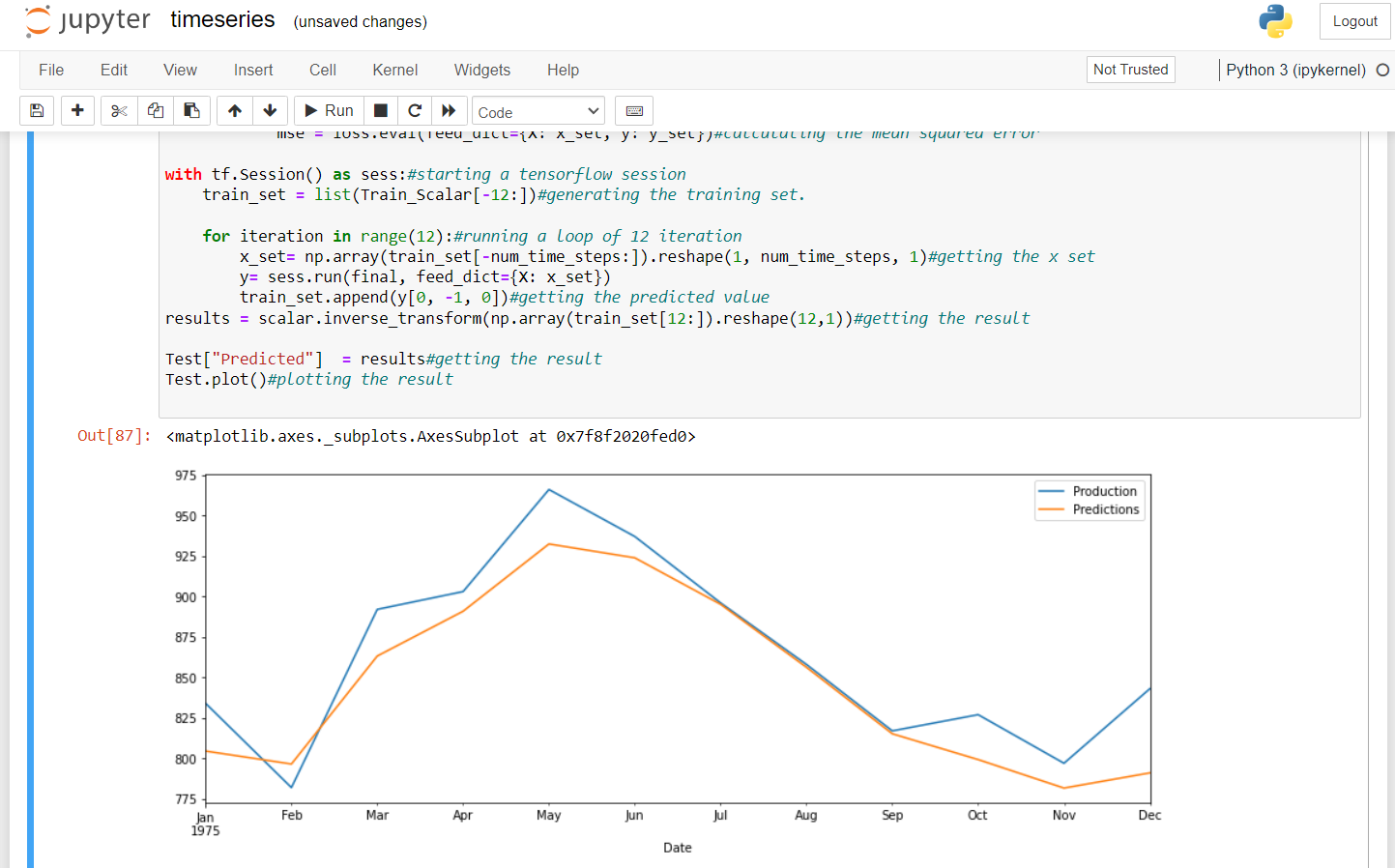
results = scalar.inverse_transform(np.array(train_set[12:]).reshape(12,1))#getting the result
Test["Predicted"] = results#getting the result
Test.plot()#plotting the result
Summary
In this Machine Learning project, we built a time series project. For this, we used RNN and LSTM. We hope you have learned something new from this project.